월요일! 2주차 아침퀴즈를 마치고 머신러닝을 달려본다!!
- 딥러닝[Deep learning == Deep neural networks == Multilayer Perceptron(MLP)]
- 딥러닝의 역사
- AND, OR 문제를 논리회귀로 풀고 표현한 모양을 퍼셉트론(Perceptron)이라 명칭
- 선형회귀로 풀지 못하는 XOR 문제 발생
- Multilayer Perceptrons (MLP)라는 개념을 도입했으나 당시 기술로는 불가능
- Backpropagation(역전파) : 출력에서 Error(오차)를 발견하여 뒤에서 앞으로 점차 조절하는 방법
- 역전파 알고리즘 발견으로 XOR 문제를 해결

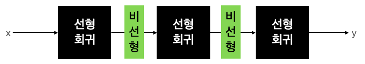
- Deep Neural Networks 구성 방법(딥러닝의 네트워크 구조)
- Layer(층) 쌓기 : 마름모 형태

- Hidden layers : 완전연결 계층 (Fully connected layer = Dense layer)
- 활성화 함수 위치

- Baseline model(베이스라인 모델)의 튜닝
- 히든레이어의 노드 개수를 늘려 너비를 튜닝하는 방법
- 히든레이어의 개수를 추가하여 깊이를 튜닝하는 방법
- 딥러닝의 용어
- batch : 데이터셋을 작은 단위로 쪼개서 학습을 시키는데 쪼개는 단위
- iteration : 1,000만개의 데이터셋을 1,000개 씩으로 쪼개어 10,000번을 반복하는 과정
- epoch : 전체 데이터셋을 한 번 도는 주기

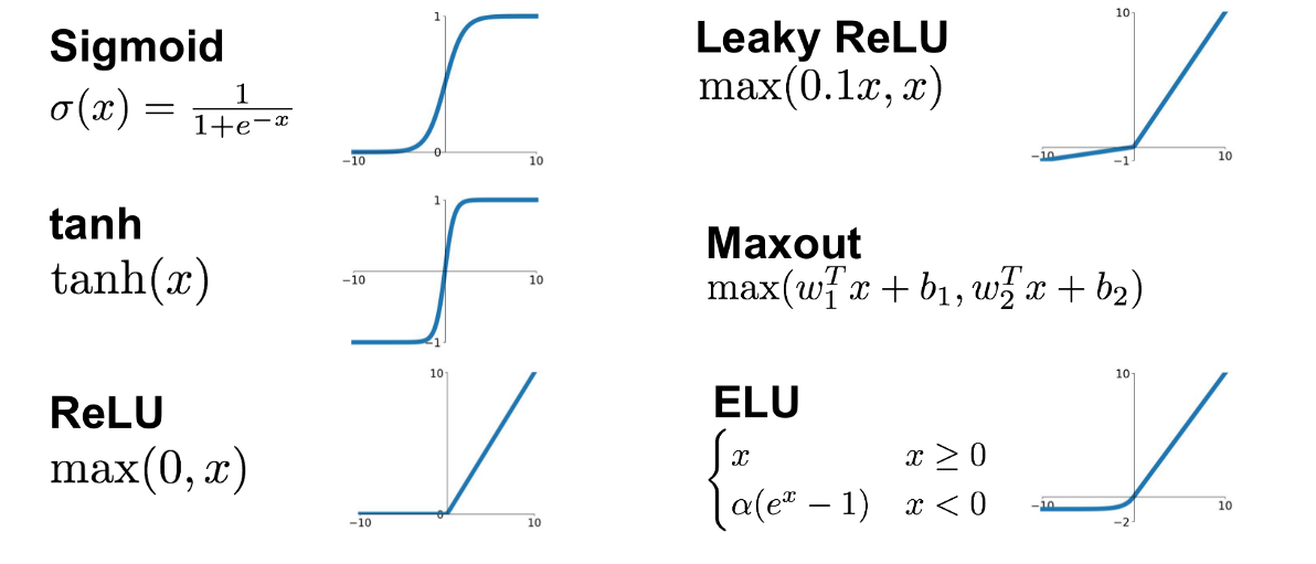
- Activation functions (활성화 함수) : 임계치(Threshold)를 넘어야 다음 단계로 활성화(비선형함수=시그모이드)
- ReLU(렐루) : 학습이 빠르고, 연산 비용이 적고, 구현이 간단
- Overfitting, Underfitting (과적합, 과소적합), best fit
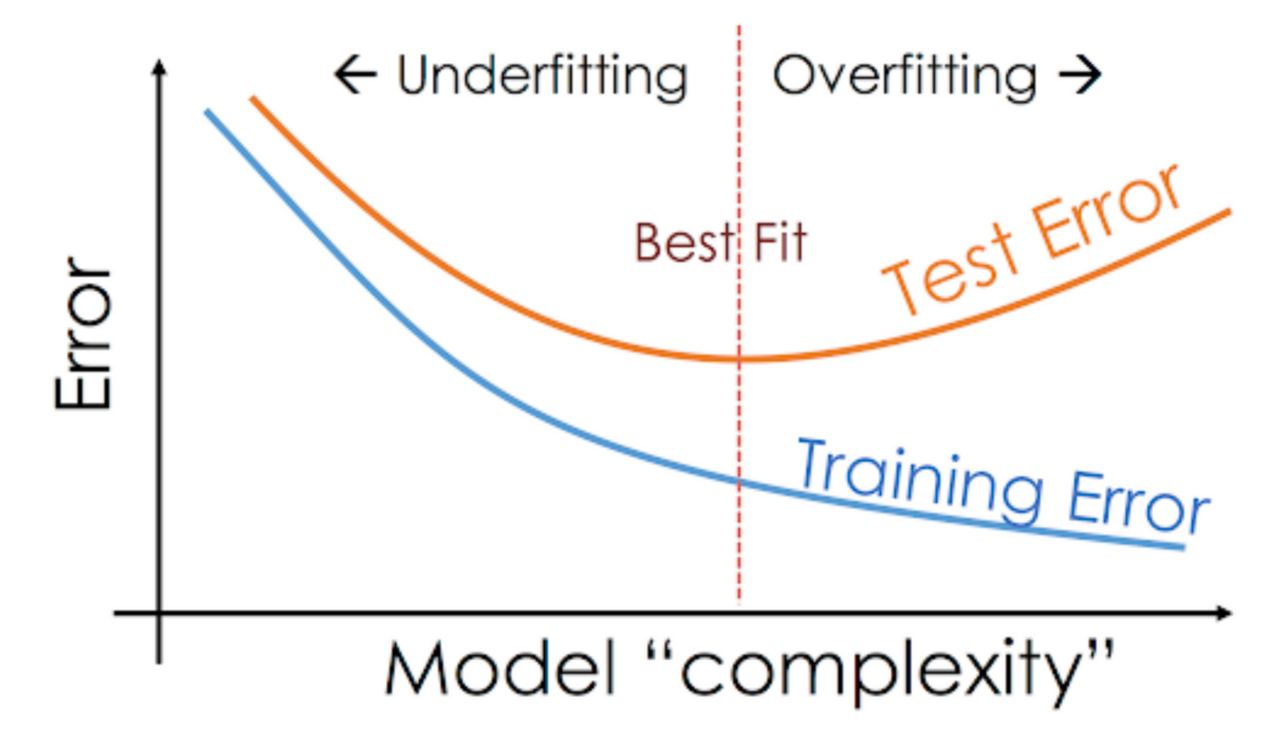
- 오버피팅을 해결하는 스킬
- Data augmentation (데이터 증강기법) : 한개의 데이터를 가공하여 데이터 더 모으기 - 가장 좋은 방법
- Dropout (드랍아웃) : 노드를 없애버림 - 가장 간단한 방법
- Ensemble (앙상블) : 여러개의 딥러닝 모델에서 나온 출력값을 기반으로 투표 - 파워소스를 많이 차지
- Learning rate decay (Learning rate schedules) : lr을 점차적으로 줄여서 진행하는 방법 - 실무에서도 자주 쓰는 기법
- Keras에서는 tf.keras.callbacks.LearningRateScheduler() 와 tf.keras.callbacks.ReduceLROnPlateau() 를 사용
# 라이브러리 임포트 약어
from tensorflow.keras.models import Model
from tensorflow.keras.layers import Input, Dense
from tensorflow.keras.optimizers import Adam, SGD
import numpy as np
import pandas as pd
import matplotlib.pyplot as plt
import seaborn as sns
from sklearn.model_selection import train_test_split
from sklearn.preprocessing import StandardScaler
from sklearn.preprocessing import OneHotEncoder

# 데이터프레임 로드
train_df = pd.read_csv('mnist_train.csv')
test_df = pd.read_csv('mnist_test.csv')

# 라벨 분포 확인
plt.figure(figsize=(16, 10))
sns.countplot(train_df['label'])
plt.show()

# 전처리 - 입출력 나누기
train_df = train_df.astype(np.float32)
x_train = train_df.drop(columns=['label'], axis=1).values
y_train = train_df[['label']].values

test_df = test_df.astype(np.float32)
x_test = test_df.drop(columns=['label'], axis=1).values
y_test = test_df[['label']].values

# 전처리 - 데이터 미리보기
index = 1
plt.title(str(y_train[index]))
plt.imshow(x_train[index].reshape((28, 28)), cmap='gray')
plt.show()

# 전처리 - 1-hot 인코딩
encoder = OneHotEncoder()
y_train = encoder.fit_transform(y_train).toarray()
y_test = encoder.fit_transform(y_test).toarray()

# 전처리 - 일반화
x_train = x_train / 255.
x_test = x_test / 255.

# 네트워크 구성
input = Input(shape=(784,))
hidden = Dense(1024, activation='relu')(input)
hidden = Dense(512, activation='relu')(hidden)
hidden = Dense(256, activation='relu')(hidden)
output = Dense(10, activation='softmax')(hidden)

model = Model(inputs=input, outputs=output)

model.compile(loss='categorical_crossentropy', optimizer=Adam(lr=0.001), metrics=['acc'])

# 모델 학습
history = model.fit(
    x_train,
    y_train,
    validation_data=(x_test, y_test),
    epochs=20
)

# 그래프 그려보기(로스, 정확도)
plt.figure(figsize=(16, 10))
plt.plot(history.history['loss'])
plt.plot(history.history['val_loss'])

plt.figure(figsize=(16, 10))
plt.plot(history.history['acc'])
plt.plot(history.history['val_acc'])
'Python > Machine Learning' 카테고리의 다른 글
| Til - 24day (0) | 2022.05.19 |
|---|---|
| Til - 23day (0) | 2022.05.17 |
| Wil - 4week (0) | 2022.05.16 |
| Til - 21day (0) | 2022.05.13 |
| Til - 20day (0) | 2022.05.12 |


